Written by Allen Wyatt (last updated August 13, 2022)
This tip applies to Excel 2007, 2010, 2013, 2016, 2019, Excel in Microsoft 365, and 2021
Lana has a huge list of book titles in column A. Some of the book titles are in bold, but most are regular. If she sorts the list, Lana would like the bold titles to be sorted as a group first, followed by the non-bold titles. She wonders if the "bold/not bold" status of a cell can be factored into a sort.
Excel doesn't provide a way to take bold into account in sorting. There are, however, several ways you can tackle the task. Different approaches are addressed in the following sections.
Using a Color
The first approach relies on the fact that even though you can't sort by bold status, you can sort based on color. So, one way to sort the bold cells first is to follow these steps:
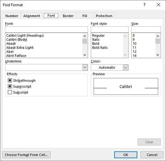
Figure 1. The Font tab of the Find Format dialog box.
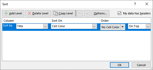
Figure 2. Sorting based on cell color.
At this point, the colored cells that contain bold titles are at the top of your sorted list. If you want to, you can select those cells and, using the Fill Color tool on the Home tab of the ribbon, remove the fill color.
Using a Helper Column
Another approach is to utilize a helper column that can indicate whether the book title is in bold or not. This can be done most easily using a defined name. Display the Formulas tab of the ribbon and click the Define Name tool. Excel displays the New Name dialog box. You want define a name that uses these specifications:
Name: CheckBold
Scope: Workbook
Refers To: =GET.CELL(20,Sheet1!$A2)
In the formula you place in the Refers To box, you should make sure that Sheet1 is the name of the worksheet you are working with, and that $A2 is the cell of the first title in column A. (If your titles column has no header cell in A1, then you should change $A2 to $A1 in the formula.) When you are done, click OK to define the formula and close the New Name dialog box.
Now, assuming that your worksheet only has values in column A (the book titles), select the cell in column B that is just to the right of the first book title. (If you have a heading in cell A1, then your first book title is in cell A2, so you should select the cell to its right, which is B2.) You want to put the following into that cell:
=CheckBold
What you should see is either TRUE or FALSE, based on whether the title to the left of the cell is bold or not. This works because the GET.CELL function is being used to return whether the cell is bold or not. You can copy this formula down as many cells as necessary, and you end up with a series of TRUE/FALSE values in column B.
Now you can perform your sort using the value in column B as the first sort key and the title in column A as the second sort key. When you specify the helper column (B) as the primary sort key, make sure you sort by Largest to Smallest, as this will place the bold titles at the top of the final sorted list.
Using a Macro
A variation on the previous approach is to convert the approach into a macro. This is a great choice if you need to do the sorting often, plus it precludes the need to define any names. The following macro adds a helper column to the left of column A (so that your data table gets moved to the right), sets a value in the new helper column to indicate if the title is bold or not, sorts the data, and then deletes the helper column.
Sub SortBold()
    Dim J As Long
    Dim lNumRows As Long
    Dim lFirstData As Long
    Dim sSortRange As String

    ' Change the following to the row number of the first title in the table.
    lFirstData = 2

    lNumRows = Cells(Rows.Count, 1).End(xlUp).Row

    ' Change the following range if there is more than one column in the table.
    ' The ending column in the range should be one greater than the number of
    ' columns in the table.
    sSortRange = "A" & lFirstData & ":B" & lNumRows

    Application.ScreenUpdating = False
    ' Add the helper column and populate it
    Range("A1").EntireColumn.Insert
    For J = lFirstData To lNumRows
        If (Range("B" & J).Font.Bold) Then
            Range("A" & J) = 0
        Else
            Range("A" & J) = 1
        End If
    Next J

    ' Sort the data
    Range(sSortRange).Sort _
      Key1:=Range("A1"), Order1:=xlAscending, _
      Key2:=Range("B1"), Order2:=xlAscending, _
      Header:=xlNo

    ' Delete the helper column
    Range("A1").EntireColumn.Delete
    Application.ScreenUpdating = True
End Sub
Note that there are only two things you need to change in the macro in order to make it useful for yourself. First, you need to make sure that lFirstData is set to the number of the first row that contains a book title. In the example shown above, it is set to 2 because the first row contains column headers. The second thing to note is the specification of the range to be sorted. This is stored in the sSortRange variable, and as shown only sorts the range of A2 through B-whatever (depends on the number of rows in the table). If you have data in other columns, then you'll need to change "B" to account for those columns. So, if you have data in columns A through G, then you would change the range designation to this:
sSortRange = "A" & lFirstData & ":H" & lNumRows
Note that the ending column should always be one greater than the number of columns you actually use. This is because, of course, the macro adds a helper column which expands the range of cells in the table.
Other Possible Approaches
You may want to rethink your approach to your data. For instance, consider why you are making some book titles bold. Perhaps you want to note some attribute of the title, such as its best-seller status, its importance, or some other attribute. In these cases, you should seriously consider adding a column to your data table that is used to denote the attribute. For instance, you might add a column used to indicate whether the title is a best-seller. In this way, you don't need to make your book titles specifically bold, but you could use a conditional format to add the special formatting to the title based on the setting within the attribute column. This would also make sorting much easier, as you could sort first on the attribute column and then on the book title column.
If you don't want to add additional columns, consider not using bold for your special titles, but instead choose a different font color or a different cell color. Doing so allows you to sort the cells directly, as done earlier in this tip.
Finally, you can always look to a third-party add-in to do your special sorting. One very popular add-in is ASAP Utilities, and it includes an expanded sorting capability that will allow you to sort based on whether text is bold or not.
ExcelTips is your source for cost-effective Microsoft Excel training. This tip (12953) applies to Microsoft Excel 2007, 2010, 2013, 2016, 2019, Excel in Microsoft 365, and 2021.

Create Custom Apps with VBA! Discover how to extend the capabilities of Office 2013 (Word, Excel, PowerPoint, Outlook, and Access) with VBA programming, using it for writing macros, automating Office applications, and creating custom applications. Check out Mastering VBA for Office 2013 today!
Government and industrial organizations often use a numbering system that relies upon a number both before and after a ...
Discover MoreWhen you sort data in a worksheet, you don't need to sort everything at once. You can sort just a portion of your data by ...
Discover MoreWhen entering information into a worksheet, you may want it to always be in a correctly sorted order. Excel allows you to ...
Discover MoreFREE SERVICE: Get tips like this every week in ExcelTips, a free productivity newsletter. Enter your address and click "Subscribe."
There are currently no comments for this tip. (Be the first to leave your comment—just use the simple form above!)
Got a version of Excel that uses the ribbon interface (Excel 2007 or later)? This site is for you! If you use an earlier version of Excel, visit our ExcelTips site focusing on the menu interface.
FREE SERVICE: Get tips like this every week in ExcelTips, a free productivity newsletter. Enter your address and click "Subscribe."
Copyright © 2024 Sharon Parq Associates, Inc.
Comments